
Overview
- This blog post demonstrates a complex simulation workflow for footwear design in Rhino Grasshopper. We show how external data (from pressure sensors) can be incorporated in a stress simulation to study footwear deformation for multiple positions in the stance.
- The workflow also demonstrates how feedback from simulation can be used to optimize the footwear design for performance. Specifically, a gyroid lattice is sized based on the stress values.
- Intact.Simulation can be seamlessly integrated in your design workflows and allow you to explore a much larger design space to find innotive high performance solutions previously not feasible.
Motivation
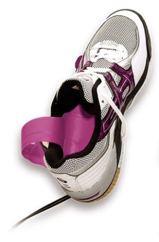
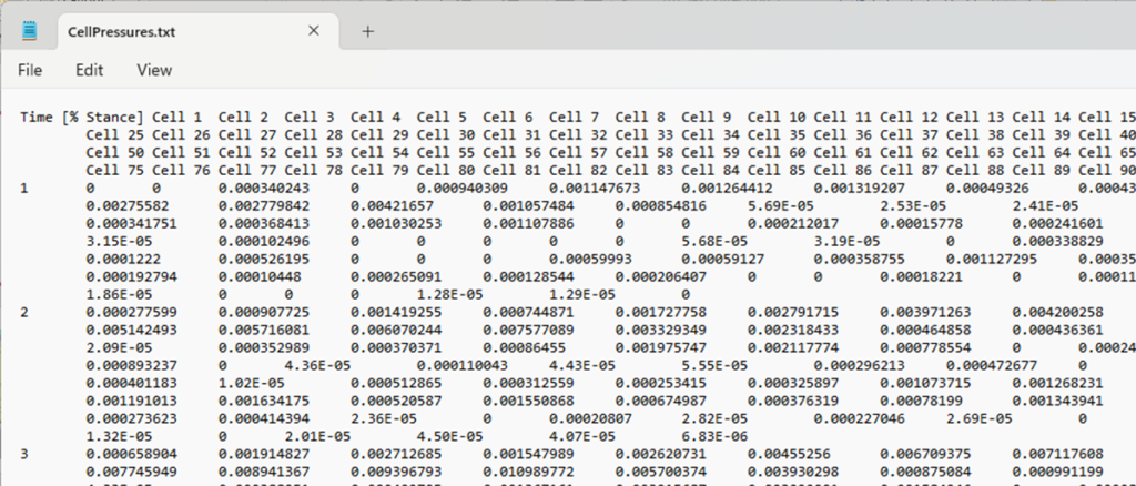
A client is working on the design of a new shoe sole based on acquired plantar pressure data. The data comes in the form of an Excel spreadsheet with rows corresponding to pressure readings at different percentages of a stance, starting with heel arrival and ending with toe departure. The coordinates of the pressure sensors are described in a separate spreadsheet. Our task is to read the external pressure data and map it to boundary conditions on the sole model. We then go the extra mile and use simulation results to design a hypothetical shoe sole with a gyroid infill whose thickness is governed by von Mises stress.
Parsing input
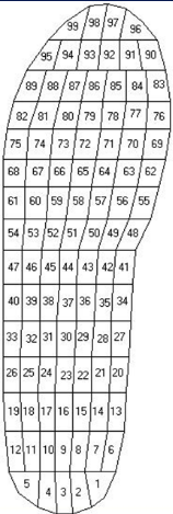
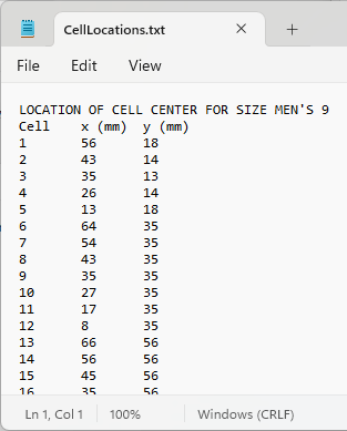
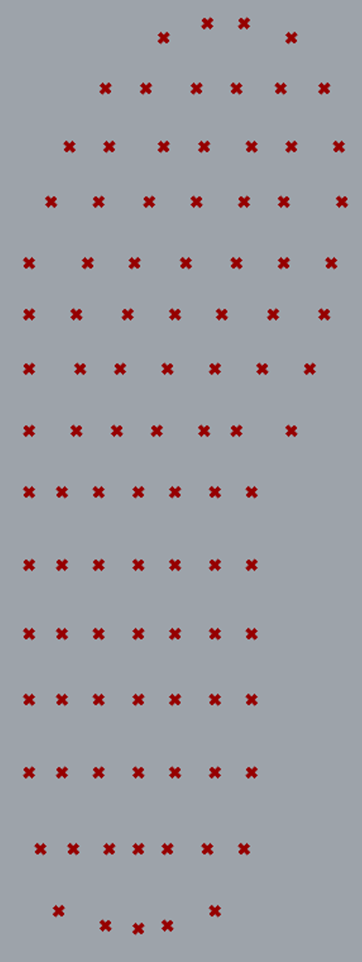
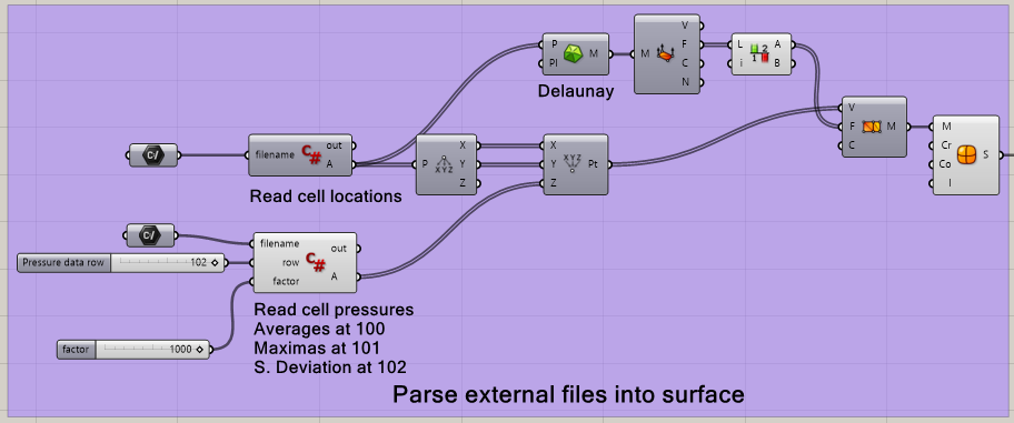
The pressure input consists of two tables: one, a table of sensor locations; and two, a table of sensor readings. Exported from Excel into Notepad, the resulting tab-delimited text files can be easily parsed using C# scripting components in Grasshopper. Within Excel, additional properties of the pressure data are easily computed (e.g. average, maxima, standard deviation) and exported to the text file.
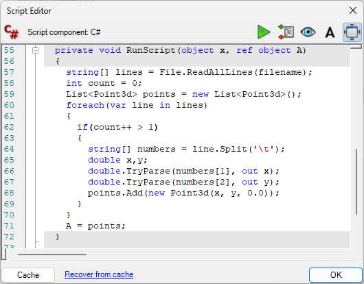

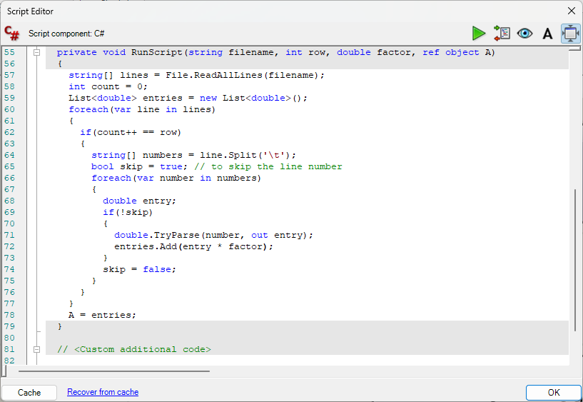
Pressure data is read using a Grasshopper C# block that parses a selected row into a list of pressure values.
Pressure data is read using a Grasshopper C# block that parses a selected row into a list of pressure values.
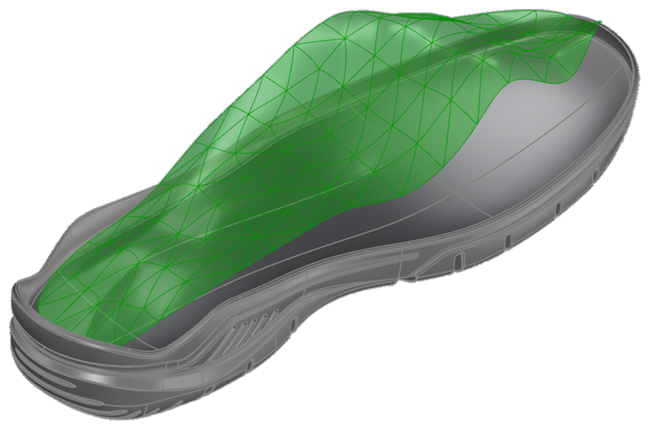
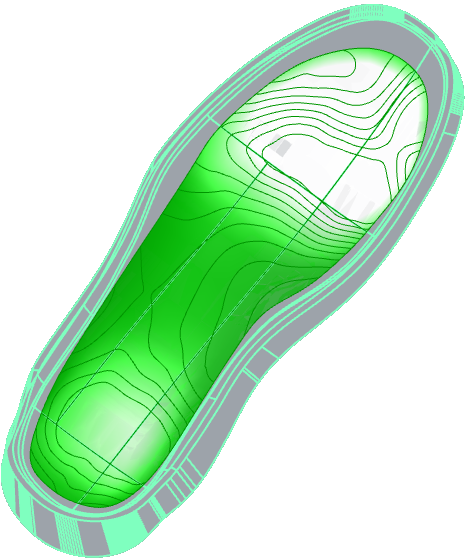
We add structure to the sensor locations using Delaunay triangulation. By decomposing the vertices of the resulting mesh and replacing the z-coordinate of each vertex with the corresponding (scaled) pressure value we get a visual representation of the pressure distribution. This can be done for any row of the data. For downstream processing, the thus-deformed mesh is smoothed by conversion to a subdivision surface.
For simulation, we want to take into account the spatial variation in the pressure. Intact.Simulation for Grasshopper doesn’t have a way to do this directly so we’ll have to get creative. The Pressure Block accepts a list of surfaces to which a single pressure magnitude may be applied. We can therefore approximate the pressure distribution by a set of overlapping surface regions, each with a uniform pressure applied. The final pressure distribution will be the sum of all contributing surface segments.
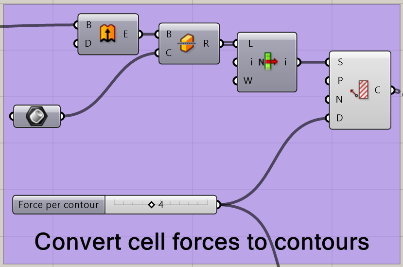
We generate the surface regions by contouring the pressure distribution and using the contours to trim the sole upper surface into the desired overlapping regions. The Grasshopper network to generate the contours from the pressure distribution surface is shown below. The pressure surface is extruded to create a solid that is split into upper and lower pieces along the plane Z=0. The upper half is contoured to produce planar curves akin to a topographical map of the pressure distribution. Extruding the pressure surface to create a solid ensures the contours are closed curves.
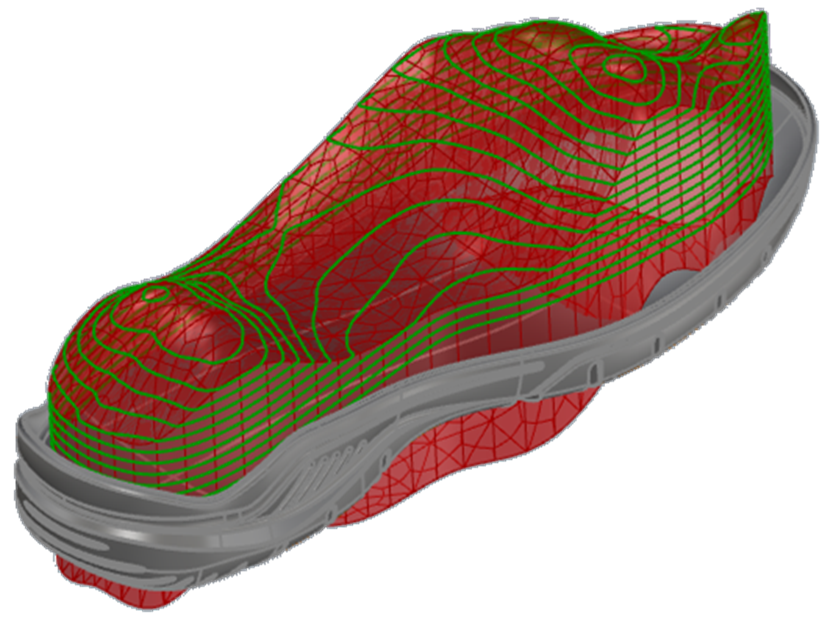
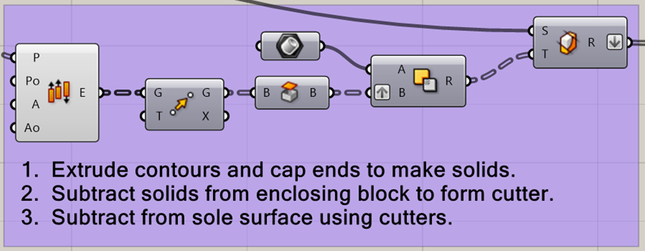
Akin to the extrusion of the pressure surface, the pressure contours are extruded into solids that intersect the upper surface of the sole. These solids are then used to trim away those portions of the sole surface that have pressures less than each solid’s corresponding pressure level.
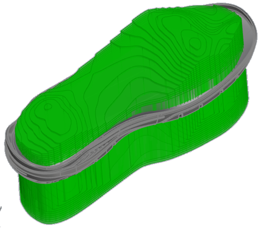
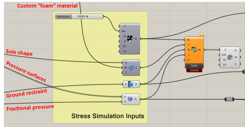
At this point running a simulation is simply a matter of assembling the pieces. A custom material is created with properties of a high density foam. This is applied to a solid model of the sole to create a simulation component. The bottom surface of the sole is restrained as if contacting the floor. Using a modest resolution of 50k elements we compute the displacement field for a range of positions in the stance, with each simulation taking around 6 seconds.
Using Simulation to Drive Design
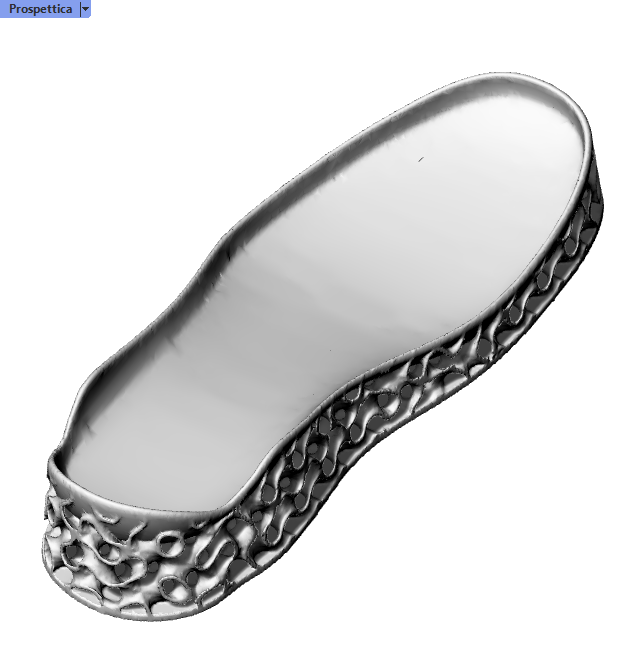
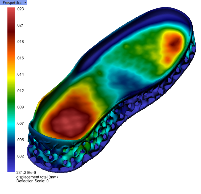
Now we’ll use simulation results to construct a unique design in two stages. In the first stage we build a sole consisting of upper and lower skins connected by a gyroid infill. On this model we run simulation to determine the stress distribution in the gyroid. In the second stage we sample the von Mises stress over the gyroid skeleton and increase the gyroid thickness where the stress is relatively high. A second run of simulation reveals the effect of the modified infill.
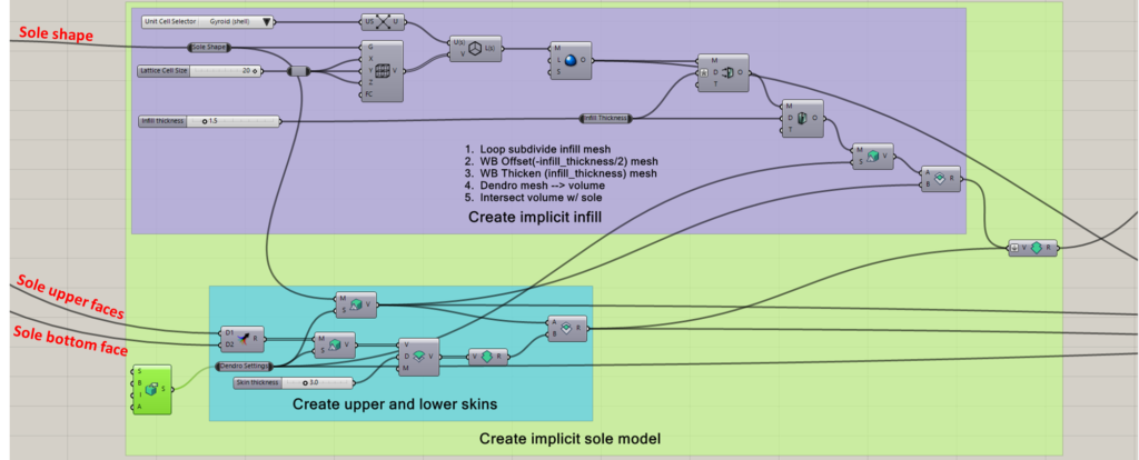
The first stage of simulation for design re-uses most of the simulation setup from the earlier. In this stage of simulation the geometry of the sole component is replaced by a VDB model constructed by converting the upper and lower faces of the sole into Dendro implicit models that are offset by an amount equal to the desired skin thickness (3 mm in this case). Crystallon is used to to create the skeleton of the gyroid infill. This skeleton is smoothed using one iteration of Weaverbird’s Loop subdivision. The resulting mesh is offset, thickened, and converted to an implicit model using Dendro. A few more Dendro Boolean operations combine this infill with the skins and trim away everything exterior to the original sole. The final implicit sole model is written to a VDB file for input into simulation.
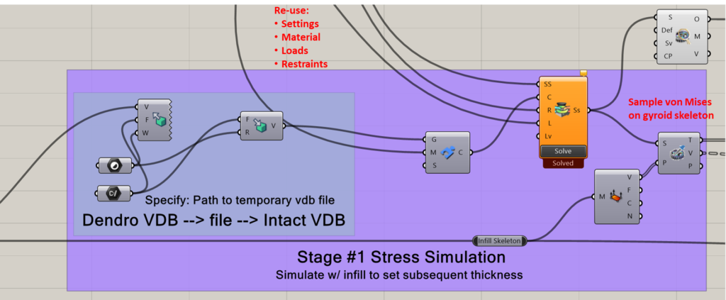
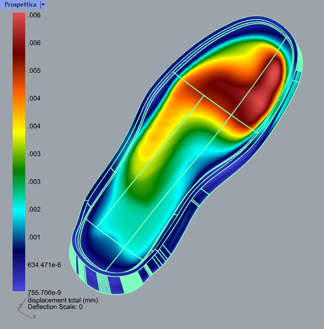
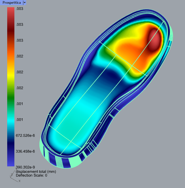
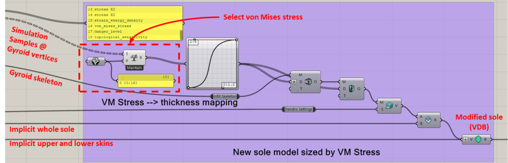
In a second stage we use the von Mises stress field to adjust the gyroid size. To do this, the solution fields are sampled at the vertices of the gyroid skeleton. The von Mises stress component is extracted and a graph mapper component maps the range of von Mises stresses to thicknesses ranging from 1.2 mm to 5 mm. These thickness values are used to drive Weaverbird offset and mesh thicken blocks applied to the mesh skeleton. A few Dendro operations and we’re ready for a final round of simulation (duplicate Stage 1 except with the new geometry) to see the effects.
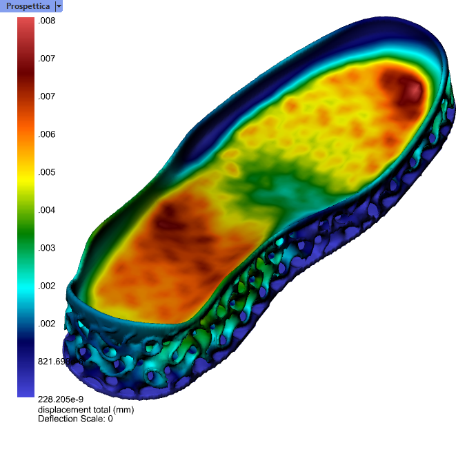
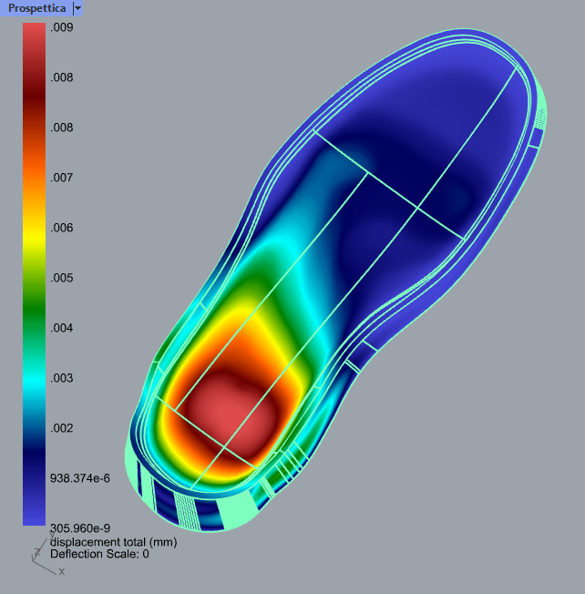
We can see from this round of simulation that this simulation-modified gyroid has a more uniform distribution of displacement and a maximum displacement 2/3 that of the basic infill. An experienced shoe designer (That’s not us!) should be able to use a similar workflow to generate entire families of shoe soles that meet particular design goals based on any simulation quantity.